(Use arrow keys to navigate slides, F11 for fullscreen)
Procedural Gas Giant Planet Textures
Stephen M. Cameron -- August 27, 2014

(Animation not computed in real time)
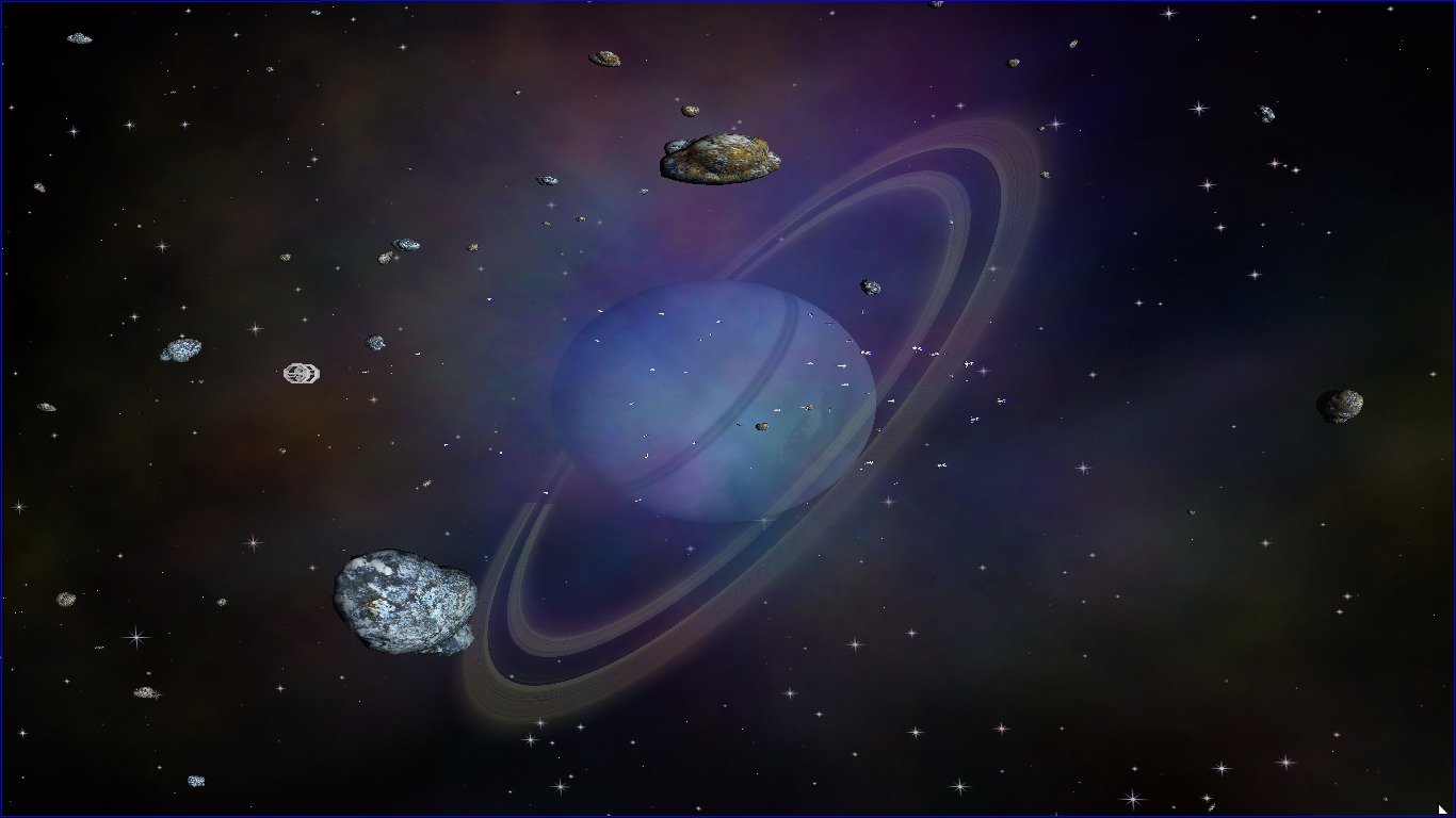
So You're Making a Space Game...
You're gonna need some planets
First attempts... Try Crazy Things Like..
First attempts... Try Crazy Things Like..
Photoshopping Marble Floor Tiles

|
---> |
|
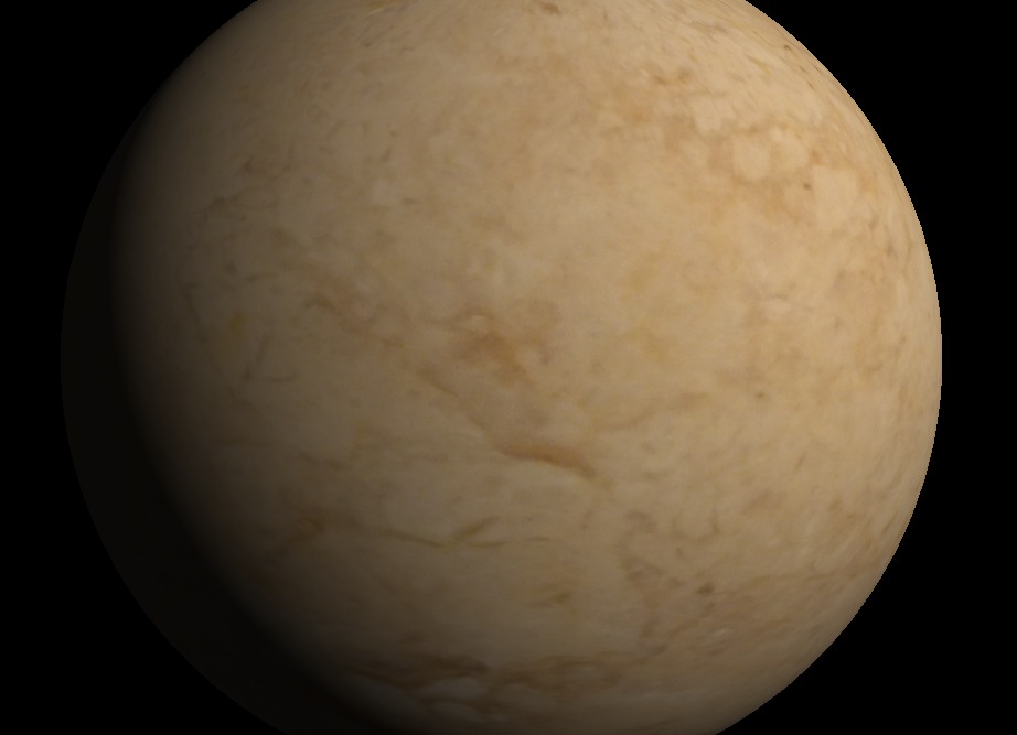
. . . which almost works.
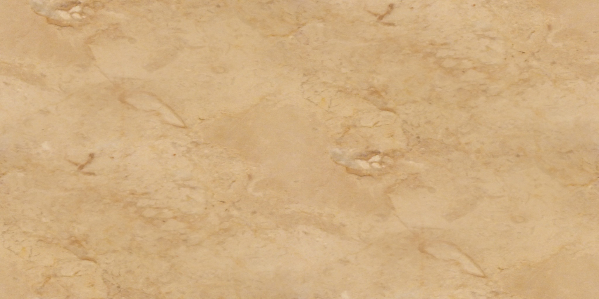
Photoshopping Marble Floor Tiles
1. Crop so it's 2x as wide as it is tall
2. Make seamless (gimp: Filters/Render/Map/Make Seamless)
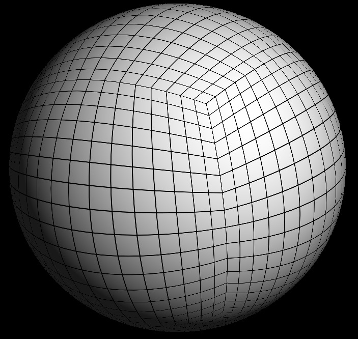
3. Run through an Equirectangular to Cubic transformation
2. Make seamless (gimp: Filters/Render/Map/Make Seamless)
3. Run through an Equirectangular to Cubic transformation
| Step 1. |
| Step 2. |
|
|
|
|
|
|
|
|
|
|
|
|
|
|
|
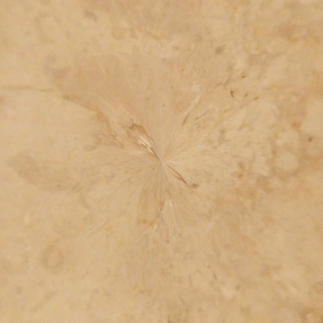
Problems with Photoshopping Marble Floor Tiles
1. Pinching at the poles (mitigate via more hand photoshopping)
Problems with Photoshopping Marble Floor Tiles
2. Time consuming manual process (mitigate somewhat with ImageMagick, etc.)
Problems with Photoshopping Marble Floor Tiles
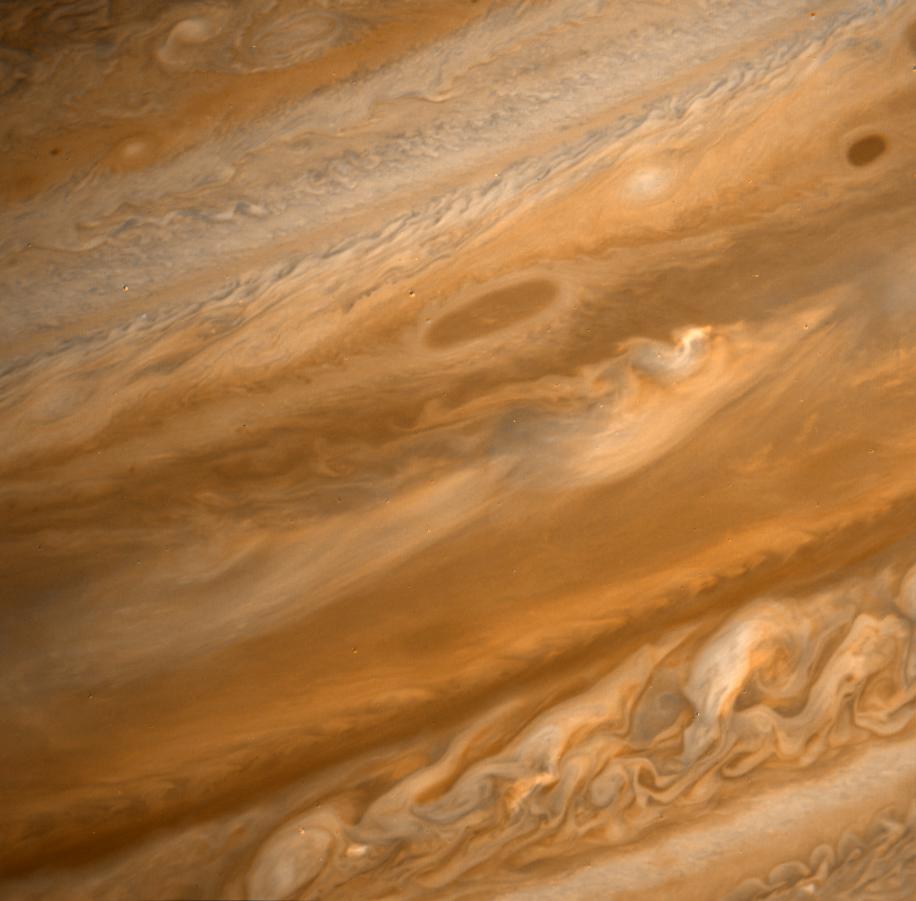
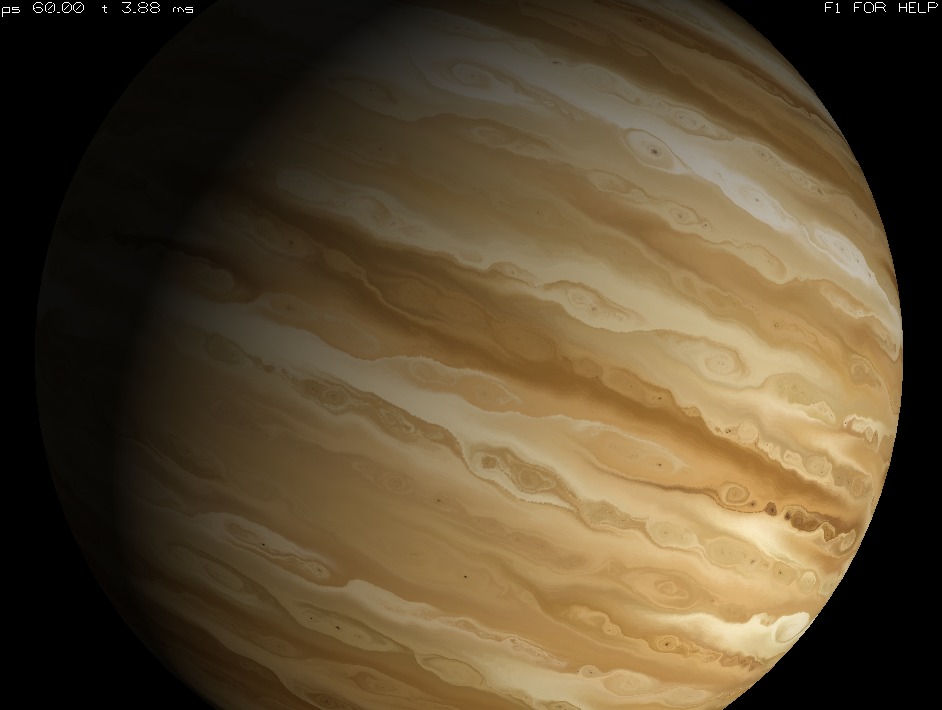
3. Just look at these photos of Jupiter from NASA.
|
|
|
Hmm. My stupid floor tiles just don't really measure up, do they?
Computational Fluid Dynamics All the Things!
Like this youtube video.
Computational Fluid Dynamics All the Things!
Oh man, that's hard. Like, really hard...
Can we cheat?
Can we cheat?
Computational Fluid Dynamics All the Things!
Yes we can.
Computational Fluid Dynamics All the Things!
Robert Bridson shows us how to cheat
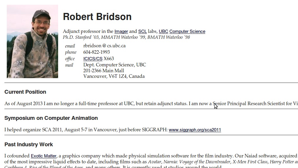
Curl Noise for Procedural Fluid Flow
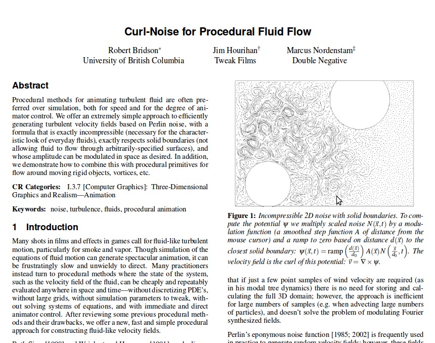
Curl Noise for Procedural Fluid Flow
In mathematical lingo, the summary of this paper is:
Take the curl of the gradient of a noise field to produce
a chaotic but divergence free velocity field.
Huh?
Take the curl of the gradient of a noise field to produce
a chaotic but divergence free velocity field.
Huh?
Curl Noise for Procedural Fluid Flow
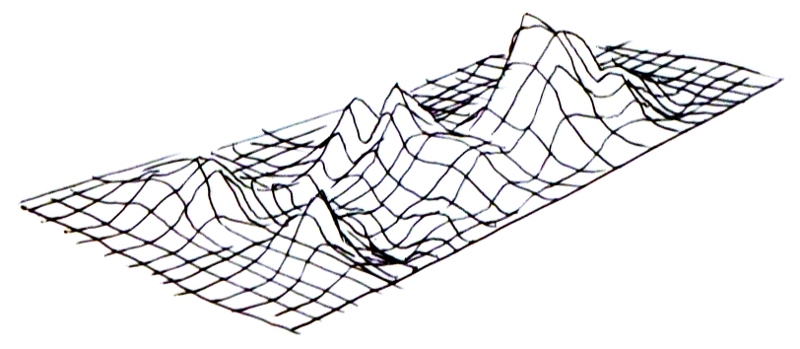
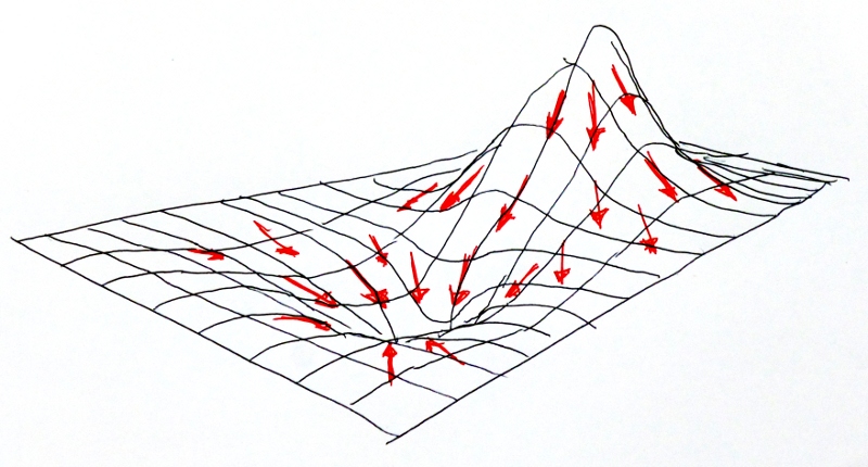
Consider a 2D Perlin (or Simplex) noise field.
Put in x and y, get out a noise value between 0.0 and 1.0;
Imagine it as a height field:
h = f(x, y); where f() is the noise function.
Put in x and y, get out a noise value between 0.0 and 1.0;
Imagine it as a height field:
h = f(x, y); where f() is the noise function.
h = f(x, y); where f() is the noise function.
Curl Noise for Procedural Fluid Flow
Update 2016-01-21: It has been pointed out to me that there
are some inconsistencies between the descriptions and the pictures. Take all these
descriptions and pictures with a grain of salt. I wrote all this shortly after I had
just gotten the program to work and didn't necessarily get all the details right in
these slides, but the basic idea is here. Consult the code to see something which
is actually known to work.
Now we can compute the gradient of the noise field wrt x and y.
That is, compute a 2D vector field where at each point the vectors
point in the direction of "most downhill" -- the direction a marble would
roll if released at that (x,y) position in the height field. The magnitude
of the vector is related to the slope of the hill, the steeper it is, the
larger the magnitude.
That field of vectors that all point in the direction of "downhill" is
the gradient of the noise field.
That field of vectors that all point in the direction of "downhill" is
the gradient of the noise field.
Curl Noise for Procedural Fluid Flow
Update 2016-01-21: It has been pointed out to me that there
are some inconsistencies between the descriptions and the pictures. Take all these
descriptions and pictures with a grain of salt. I wrote all this shortly after I had
just gotten the program to work and didn't necessarily get all the details right in
these slides, but the basic idea is here. Consult the code to see something which
is actually known to work.
* Now take the "curl" of the gradient to find the velocity field.
* Bunch of scary vector math that ultimately boils down to...
* Now take the "curl" of the gradient to find the velocity field.
* Bunch of scary vector math that ultimately boils down to...
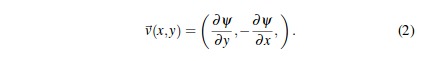
* You can visualize this as rotating all the noise gradient
vectors about the vertical (z) axis clockwise by 90 degrees.
* This can be accomplished by swapping x and y and then negating
the y component.
* v(x,y) is the velocity field, think of it as an array of vectors, indexed by x and y,
which gives you the velocity at coordinates x and y.
* Delta-Psi is the change in the noise value over some small region around x and y.
* Delta-x and delta-y define the small region over which the noise is sampled.
* To summarize, at each point (x,y) the velocity (vx, vy) is (delta-noise/delta-y, -delta-noise/delta-x), or, (vx, vy) is (slope-of-noise-in-y, -slope-of-noise-in-x).
* Delta-x and delta-y define the small region over which the noise is sampled.
* To summarize, at each point (x,y) the velocity (vx, vy) is (delta-noise/delta-y, -delta-noise/delta-x), or, (vx, vy) is (slope-of-noise-in-y, -slope-of-noise-in-x).
Curl Noise for Procedural Fluid Flow
Visualizing this process...
Curl Noise for Procedural Fluid Flow
How do we use this information in a program to make something useful?
Consider a 2D program first:
* Create a large 2D array for the velocity field, constructed as described previously
* Create a particle system to interact with the velocity field
* Each particle has a position (x,y) within the field, and a color (RGB).
* At each clock tick of the simulation each particle moves according
to the velocity field at its current location.
* Choose a method of initially coloring the particles
(e.g. map an image to the velocity field.)
* Dump a large number of particles into such a simulation at random locations
* Periodically, create an image based on the color and location
of the particles.
* Dump a large number of particles into such a simulation at random locations
* Periodically, create an image based on the color and location
of the particles.
Curly Vortex
Curly Vortex is such
a program, written in the Processing language
* It takes an image as input
* Computes a velocity field
* dumps in a bunch of particles initially colored according to input image
* Lets particles move around according to velocity field
* It takes an image as input
* Computes a velocity field
* dumps in a bunch of particles initially colored according to input image
* Lets particles move around according to velocity field
* dumps in a bunch of particles initially colored according to input image
* Lets particles move around according to velocity field
Curly Vortex
Computing the velocity field
*BTW: you can link to ranges of lines of code (e.g.: 5 - 10) on github by appending e.g.: '#L5-10', cool!
*BTW: you can link to ranges of lines of code (e.g.: 5 - 10) on github by appending e.g.: '#L5-10', cool!
Curly Vortex
Moving and drawing the particles
Curly-Vortex output:
Curly-Vortex output:
Curly-Vortex output:
Curly-Vortex output:
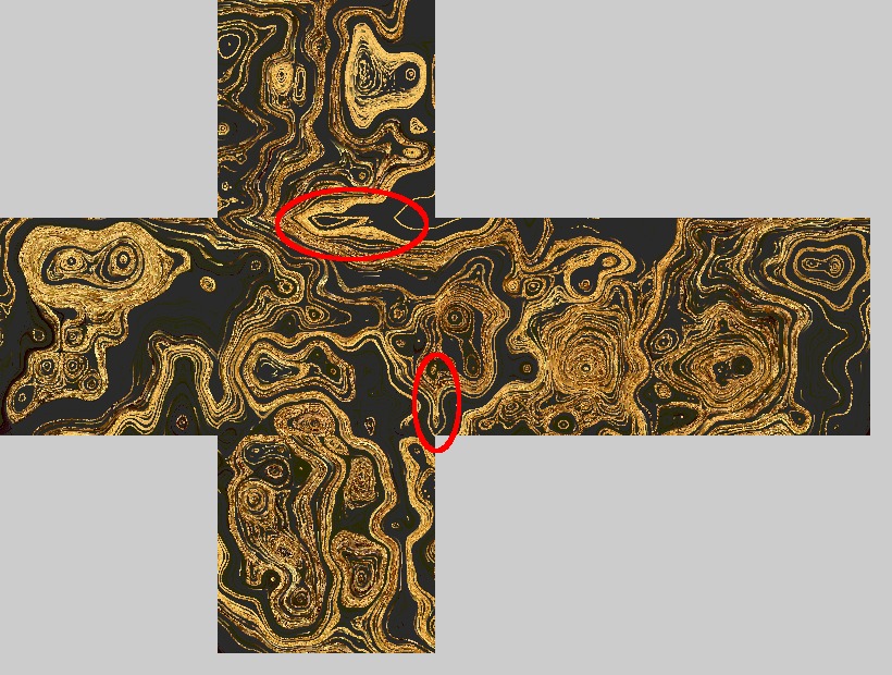
Extending Curly Vortex to 3 dimensions
Attempted to bolt together 6 instances forming 6 faces of a cube map
Particles leaving one face re-entered adjoining faces
Discontinuities in the Velocity Field! Slime in the Ice Machine!
Due to using different axes in the noise field for calculating the
velocity field of each face
Particles leaving one face re-entered adjoining faces
Discontinuities in the Velocity Field! Slime in the Ice Machine!
Due to using different axes in the noise field for calculating the
velocity field of each face
Due to using different axes in the noise field for calculating the
velocity field of each face
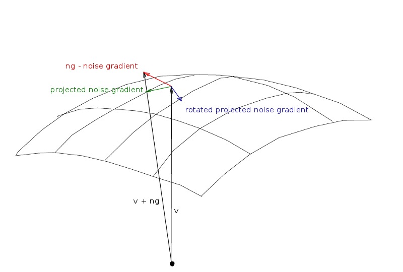
Instead, really do it in 3D proper
* Particles exist on the surface of a sphere (have x,y,z + color)
* velocity and gradient fields are in cubemapped arrays
* Noise gradient is calculated relative to surface of sphere
* velocity field is computed by rotating noise gradient 90 degrees and scaling
* Rotation direction depends on if gradient is uphill or downhill (away from or towards sphere center) No it doesn't.
* velocity field is computed by rotating noise gradient 90 degrees and scaling
* Rotation direction depends on if gradient is uphill or downhill (away from or towards sphere center) No it doesn't.
Gaseous Giganticus
Gaseous-Giganticus is such a program
Gaseous Giganticus - Computing the 6 velocity fields
Code to compute velocity fields
Multithreaded -- 1 thread per cube face (I got tired of waiting).
velocity field contained in arrays corresponding to 6 faces of a cube representing velocities on surface of a sphere (like cube mapping)
Multithreaded -- 1 thread per cube face (I got tired of waiting).
velocity field contained in arrays corresponding to 6 faces of a cube representing velocities on surface of a sphere (like cube mapping)
Gaseous Giganticus - Computing the noise gradient
Code to compute noise gradient
<--- the line numbers in this link have changed, look for the function named noise_gradient(...).
6 noise values on 3 axes are sampled in the immediate vicinity of the point of interest
6 noise values on 3 axes are sampled in the immediate vicinity of the point of interest
Gaseous Giganticus - Computing the 6 velocity fields
Code to compute velocity from noise gradient
<--- the line numbers in this link have changed. Look for the function named update_velocity_field(...) and update_velocity_field_thread_fn().
Gaseous Giganticus - Particle motion
Code for particle motion
Particle position determines velocity field array element.
New particle position is old position plus velocity field array element.
Particle position determines velocity field array element.
New particle position is old position plus velocity field array element.
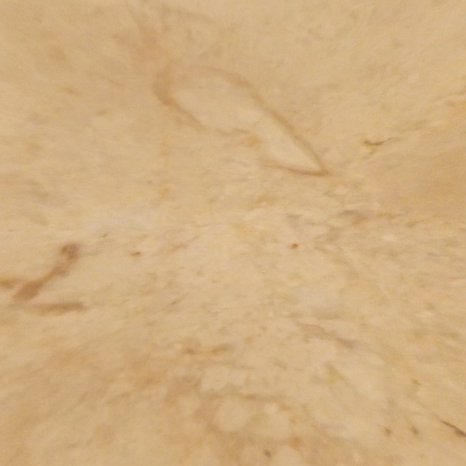
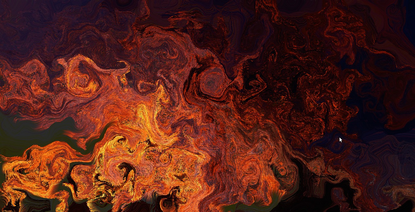
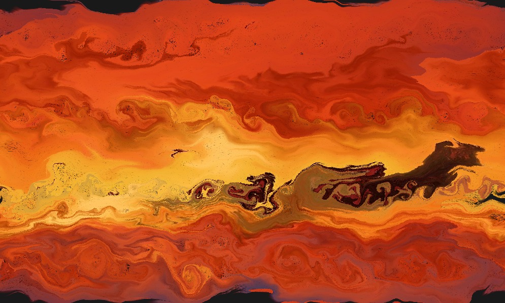
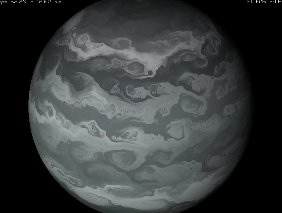
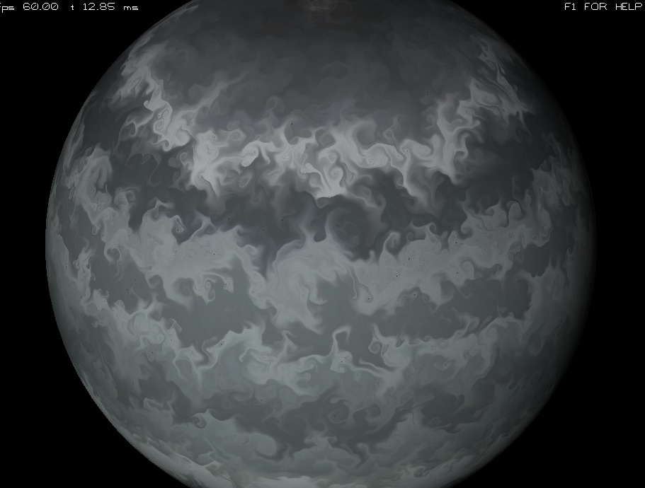
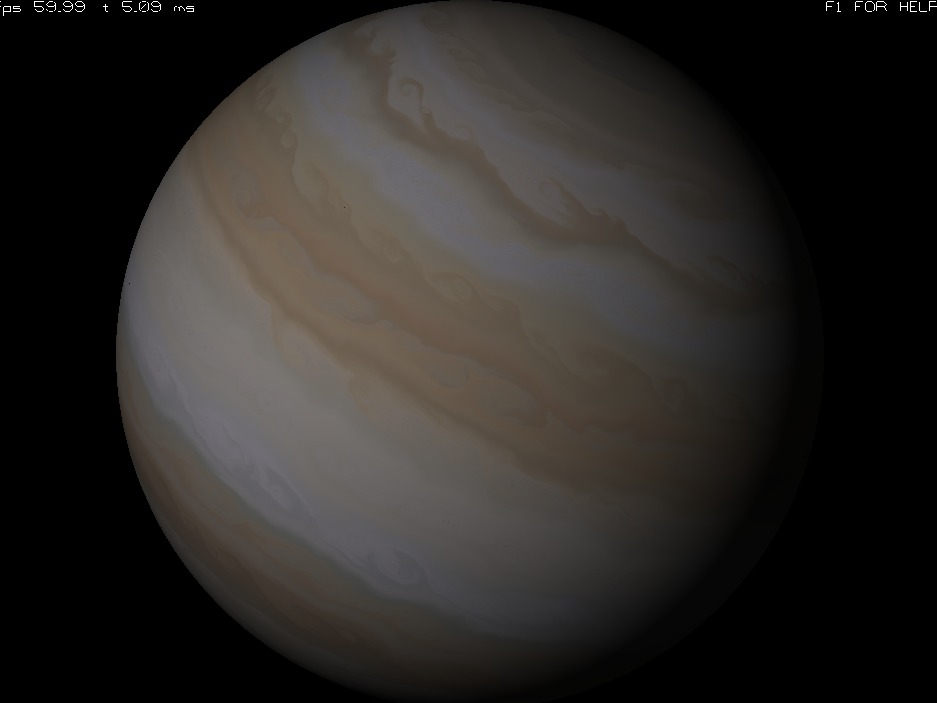
Sample Gaseous Giganticus output
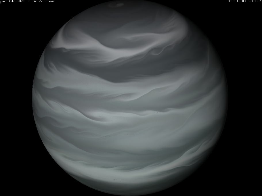
20 bands, noise-scale 0.8 velocity factor 1800
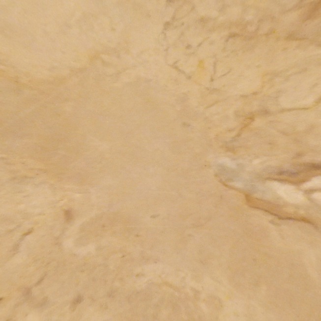
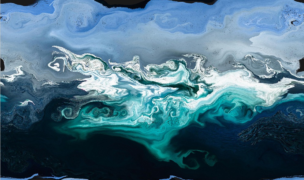
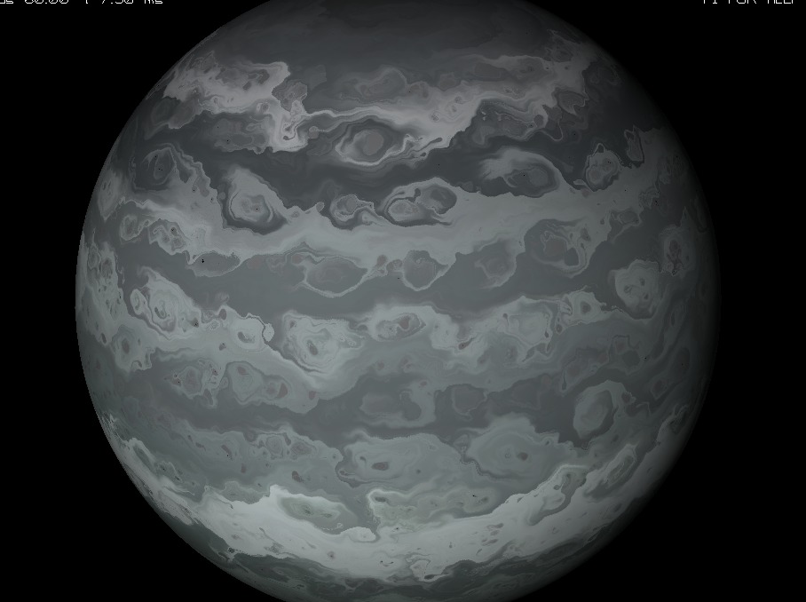
Sample Gaseous Giganticus output
20 bands, noise-scale 1.8 velocity factor 1800
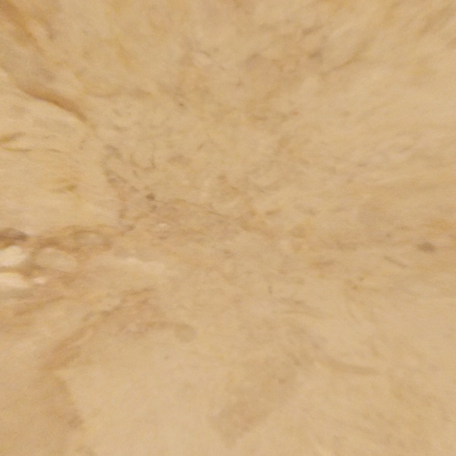
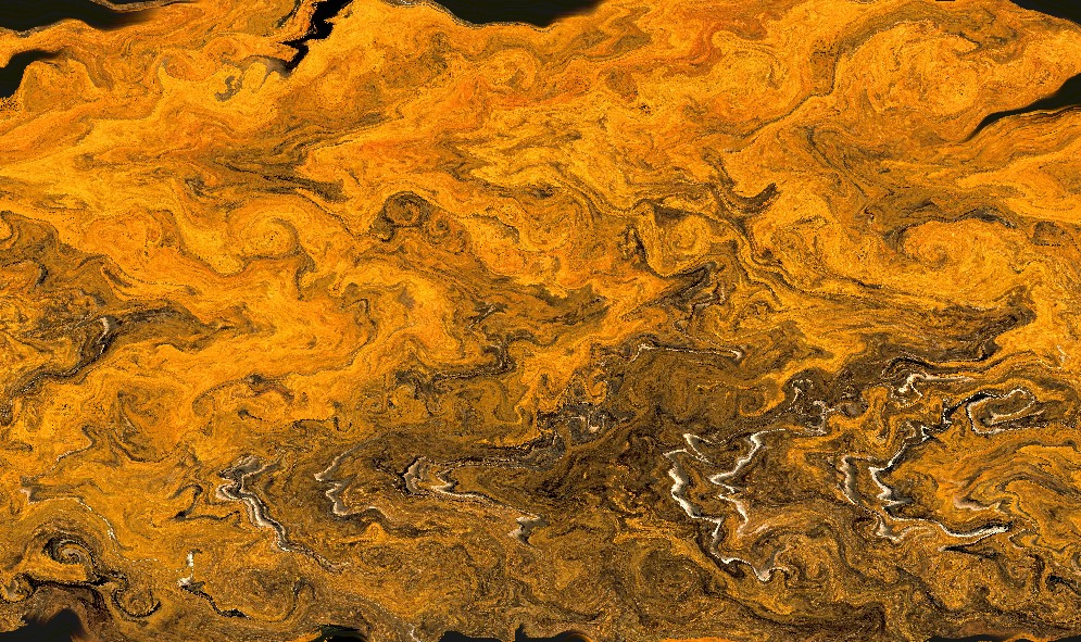
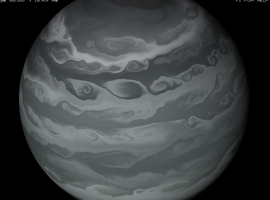
Sample Gaseous Giganticus output
20 bands, noise-scale 2.8 velocity factor 1800
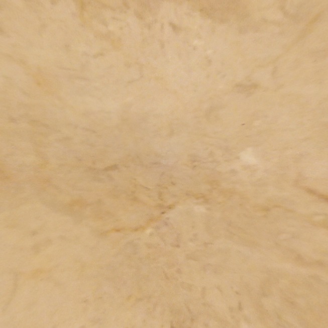
Sample Gaseous Giganticus output
20 bands, noise-scale 3.8 velocity factor 1800
Sample Gaseous Giganticus output
20 bands, noise-scale 7.0 velocity factor 1800
Sample Gaseous Giganticus output
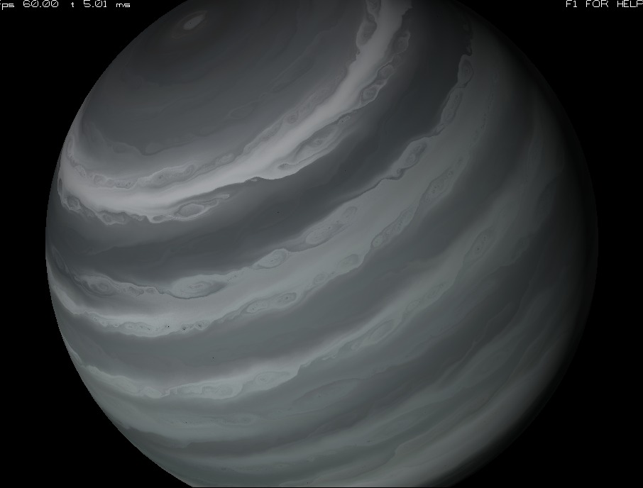
30 bands, noise-scale 3.8 velocity factor 400
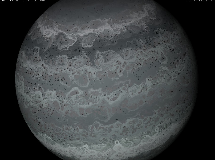
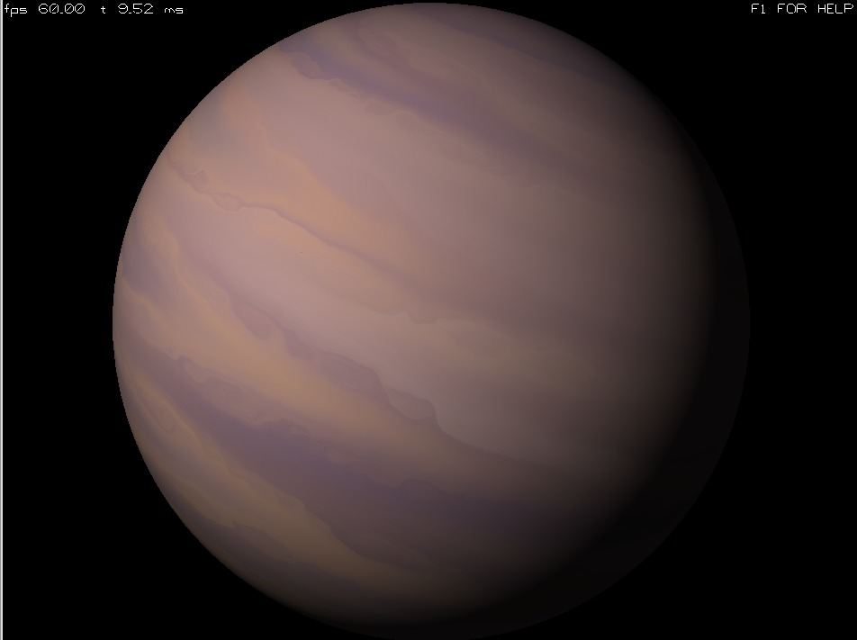
Sample Gaseous Giganticus output
0 bands, noise-scale 2.8 velocity factor 800
Sample Gaseous Giganticus output
|
--- | 
|
30 bands, noise-scale 3.8 velocity factor 500
Sample Gaseous Giganticus output
|
--- | 
|
15 bands, noise-scale 2.4 velocity factor 600
Sample Gaseous Giganticus output
|
--- | 
|
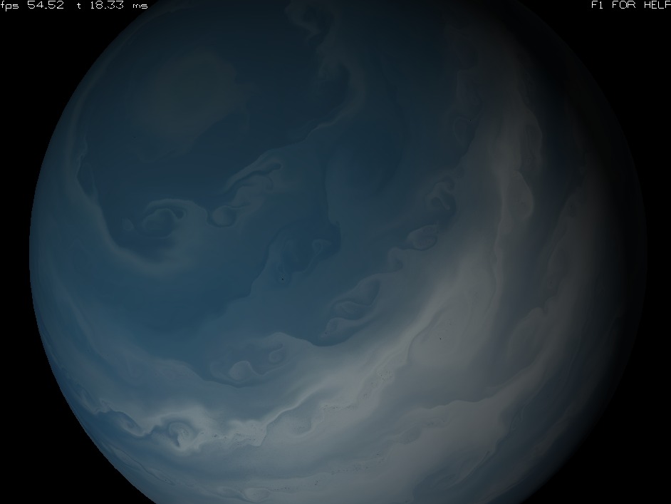
20 bands, noise-scale 2.8 velocity factor 800
Sample Gaseous Giganticus output
|
--- | 
|
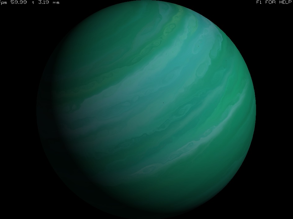
20 bands, noise-scale 2.8 velocity factor 800
Sample Gaseous Giganticus output
|
--- | 
|
20 bands, noise-scale 2.8 velocity factor 800
Links
- My github account: https://github.com/smcameron
- Curly Vortex source: https://github.com/smcameron/curly-vortex
- Gaseous-Giganticus source: https://github.com/smcameron/gaseous-giganticus
- Curl Noise for Procedural Fluid Flow by Robert Bridson, et al. (pdf)
- My github account: https://github.com/smcameron
- Curly Vortex source: https://github.com/smcameron/curly-vortex
- Gaseous-Giganticus source: https://github.com/smcameron/gaseous-giganticus
- Curl Noise for Procedural Fluid Flow by Robert Bridson, et al. (pdf)